Why Learning Rate Matters: Gradient Descent Convergence, Proven With a Closed-Form Equation (Ep:02.03)

Views: 1

A learning rate that’s too large doesn’t just train slower — it can make loss diverge to infinity, provably. Module 2 of From Zero to Agents derives the exact convergence condition for gradient descent and verifies it in Python.

Episode 02.02 ended with two questions: does gradient descent reliably keep improving forever, or can it overshoot? And what could go wrong if the learning rate is too large or too small? Both questions have exact, provable answers for a simple enough case — and working through that case gives real intuition for something every ML practitioner has felt but rarely sees derived: why a “too large” learning rate doesn’t just train a little worse, it can make training explode.

1. Theory: what repeating the update actually does

1.1 The general update rule. Gradient descent, iterated, is just Episode 02.02’s single step, repeated:

$$\theta_{t+1} = \theta_t – \eta \, \nabla L(\theta_t)$$

Read the notation the way it appears in essentially every optimization paper: $\theta_t$ (theta) is the parameter’s value at step $t$, $\eta$ (eta) is the learning rate — a small positive number controlling step size — and $\nabla L(\theta_t)$ is the gradient of the loss, evaluated at the current parameter value. Each step recomputes the gradient fresh, because the “downhill direction” generally changes as you move.

1.2 Convex bowls vs. real loss landscapes. For $f(x) = x^2$ — a single, smooth bowl with one minimum — gradient descent has a clean guarantee: done correctly, it converges to the minimum, no exceptions. This shape is called convex. Real neural network loss functions, once we build them properly in Module 03, are almost never this well-behaved — they have many local dips, flat plateaus, and saddle points (a landscape that’s neither a hill nor a valley depending on which direction you look), making convergence guarantees far weaker in practice. We’re deliberately starting with the convex case because it’s provable — it’s the case where we can derive, not just observe, exactly what learning rate does.

1.3 What “too large a learning rate” actually means, geometrically. A large step doesn’t just move further — on a curved surface, it can overshoot the minimum entirely and land on the other side, potentially further from the minimum than where it started. Repeat that every step, and instead of settling into the bowl, the parameter can bounce back and forth with growing amplitude — diverging to infinity instead of converging. Section 2 makes the exact boundary between “converges” and “explodes” a derivable number, not a guess.

2. Math: deriving the exact convergence condition

2.1 Setting up the recurrence. For $f(x) = x^2$, the gradient is $f'(x) = 2x$ (power rule, Episode 02.02 §2.1). Substituting into the update rule:

$$x_{t+1} = x_t – \eta \cdot 2x_t = (1 – 2\eta)\, x_t$$​

2.2 Recognizing a geometric sequence. This is exactly the recurrence for a geometric sequence — each term is the previous term times a fixed constant, here $(1-2\eta)$. Geometric sequences have a well-known closed form:

$$x_t = (1 – 2\eta)^t \, x_0$$

2.3 The exact convergence condition. A geometric sequence $r^t$ shrinks toward zero as $t \to \infty$ if and only if $|r| < 1$, stays constant if $|r|=1$, and blows up toward infinity if $|r|>1$. Applying that directly here, with $r = 1-2\eta$:

$$|1 – 2\eta| < 1 \iff 0 < \eta < 1$$

This is an exact, provable boundary for this specific function, not an empirical rule of thumb: **any learning rate strictly between $0$ and $1$ converges; any learning rate $\geq 1$ diverges or oscillates without shrinking, for this exact loss shape.** Notice too that $r = 1-2\eta$ can be negative (whenever $\eta > 0.5$) — a negative ratio means the sequence flips sign every step, oscillating back and forth across the minimum even while (if $|r|<1$) still shrinking toward it. This is the exact mechanism behind the oscillating-but-converging training curves you may have seen in real training runs — now you have the derivation for why that pattern appears at all.

3. Decoding a real equation — this is genuinely how papers write it

The update rule in §1.1, $\theta_{t+1} = \theta_t – \eta \nabla_\theta L(\theta_t)$, is close to verbatim how vanilla gradient descent (and its variants — momentum, Adam, and others we’ll meet once training is formalized in Module 03) is introduced in essentially every optimization paper and textbook. The subscript on $\nabla_\theta$​ is worth flagging explicitly since it appears everywhere and is easy to skim past: it specifies which variables the gradient is being taken with respect to (here, the parameters $\theta$ — as opposed to, say, the inputs $x$, which are typically held fixed during training). Seeing $\nabla_\theta$​ versus $\nabla_x$​ in a paper is the difference between “how the loss changes as we adjust what the model has learned” and “how the loss changes as we adjust the input” (the latter shows up in adversarial-example and input-attribution papers, a different subfield entirely) — same symbol, very different meaning, disambiguated only by that subscript.

4. Code: watching convergence, oscillation, and divergence, exactly as derived

4.1 From scratch — the closed form verified against the actual iteration

import numpy as np

def f(x): return x**2
def grad(x): return 2*x

def gradient_descent(x0, lr, steps):
    x = x0
    trajectory = [x]
    for _ in range(steps):
        x = x - lr * grad(x)
        trajectory.append(x)
    return trajectory

for lr in [0.05, 0.4, 0.9, 1.1]:
    traj = gradient_descent(10.0, lr, 10)
    closed_form = [10.0 * (1 - 2 * lr) ** t for t in range(11)]
    print(f"lr={lr}  (1-2*lr)={1-2*lr:.2f}  matches closed form? {np.allclose(traj, closed_form)}")
    print("  ", [round(v, 2) for v in traj])

lr=0.05  (1-2*lr)=0.90  matches closed form? True
   [10.0, 9.0, 8.1, 7.29, 6.56, 5.9, 5.31, 4.78, 4.31, 3.87, 3.49]
lr=0.4  (1-2*lr)=0.20  matches closed form? True
   [10.0, 2.0, 0.4, 0.08, 0.02, 0.0, 0.0, 0.0, 0.0, 0.0, 0.0]
lr=0.9  (1-2*lr)=-0.80  matches closed form? True
   [10.0, -8.0, 6.4, -5.12, 4.1, -3.28, 2.62, -2.1, 1.68, -1.34, 1.07]
lr=1.1  (1-2*lr)=-1.20  matches closed form? True
   [10.0, -12.0, 14.4, -17.28, 20.74, -24.88, 29.86, -35.83, 43.0, -51.6, 61.92]

Every single row matches the closed form from §2.2 exactly — this isn’t a simulation approximating the theory, it’s the theory, run. And the qualitative behavior is exactly what §2.3 predicted: $\eta=0.05$ converges steadily; $\eta=0.4$ converges fast (small $|r|=0.2$); $\eta=0.9$ oscillates in sign but still shrinks toward zero ($|r|=0.8<1$); $\eta=1.1$ oscillates in sign and grows without bound ($|r|=1.2>1$) — by step 10 the value has grown from 10 to over 61, still climbing.

4.2 The same story, visually

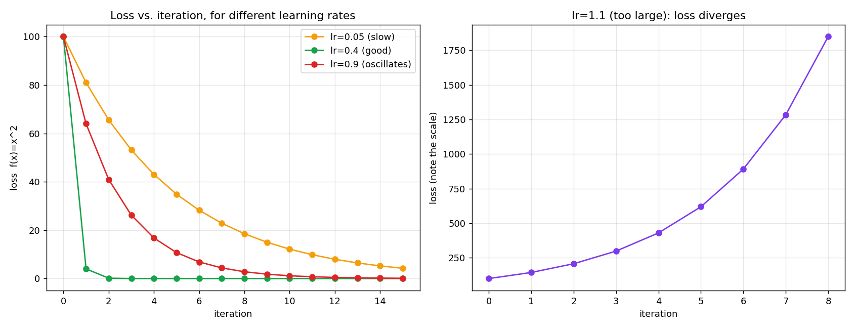
Left panel: three learning rates on the same convex loss. The small learning rate (amber) converges slowly but steadily; the well-chosen one (green) converges fast; the large one (red) visibly oscillates. Right panel: the $\eta=1.1$ case in isolation, on its own scale — note the y-axis, the loss isn’t just failing to shrink, it’s growing every single step, exactly as $|r|>1$ predicts.

4.3 A real (if tiny) training run — the 2D regression loss from Episode 02.02, iterated

x1, x2, y = 2.0, 3.0, 10.0
def L(w1, w2): return (w1*x1 + w2*x2 - y)**2
def grad(w1, w2):
    err = w1*x1 + w2*x2 - y
    return np.array([2*err*x1, 2*err*x2])

w = np.array([1.0, 1.0])
lr = 0.02
for step in range(30):
    w = w - lr * grad(*w)

print("final weights:", w, " prediction:", w[0]*x1 + w[1]*x2, " target:", y)

final weights: [1.76923077 2.15384615]  prediction: 9.999999998631619  target: 10.0

Thirty ordinary gradient-descent steps, no special tricks, and the loss (25.0 at the start, per Episode 02.02) has driven the prediction to within $10^{-9}$ of the true target. This is, in complete miniature, exactly the process that trains every model from Module 03 forward — more parameters, a more complicated loss surface, but the identical update rule, applied over and over.

5. Where this leaves us

We now have a provable answer to Episode 02.02’s closing question: gradient descent doesn’t automatically converge — it converges conditionally, and for a simple enough function, that condition is an exact, derivable number ($0 < \eta < 1$ here specifically). Real training loss surfaces are far messier than a single bowl, but the core lesson transfers directly: learning rate isn’t a minor tuning knob, it’s the difference between a provably converging process and a provably diverging one.

6. Before Episode 02.04

Everything built so far in Module 02 — vectors, matrices, gradients — deals with numbers we know exactly. But Episode 00.01’s rational-agent formula had an $\mathbb{E}[\cdot]$ (expected value) sitting right in the middle of it, and a loss function in a real training setup is usually computed over data that’s sampled, uncertain, noisy. What tool would let you reason precisely about quantities you don’t know exactly, but know something about — like “this weight update is based on a randomly sampled batch of data, not the whole dataset at once”?

That’s the on-ramp into Episode 02.04 — probability and expectation, the last major piece of Module 02 before Module 03 can properly formalize a loss function and a training loop.

Previous: Episode 02.02 — Derivatives and Gradients Next: Episode 02.04 — Probability and Expectation