Vectors, Norms, and Dot Products Explained: The Math Behind Every Embedding (Ep.02.00)

Views: 4

Every embedding, similarity score, and attention weight in modern AI comes down to vector operations. Module 2 of From Zero to Agents builds vectors, norms, and dot products from first principles, decodes a real research-paper equation, and verifies everything in Python.

Every episode so far has used vectors — one-hot vectors, co-occurrence vectors, embeddings, attention weights — without formally defining what a vector actually is, or proving why the operations we ran on them (cosine similarity, summation, dot products) behave the way they do. That was deliberate pacing, not sloppiness. Now we’re doubling back to make it precise, for a specific reason you asked for directly: once these operations are second nature — not just “code that works” but notation you can read cold — every equation in every paper that uses them stops being intimidating and starts being recognizable on sight. That’s the actual goal of this module, and this episode is where it starts.

Study pattern for this module, locked in for every episode: concept → several concrete examples → the equation stated precisely → the same thing verified in running Python code. No step skipped.

1. Theory: what a vector actually is

1.1 Two equally valid ways to picture the same object. A vector can be understood two ways, and both are correct — which one is more useful depends on the situation:

• Geometric view: a vector is an arrow with a magnitude (length) and a direction, existing in space. This is the intuitive picture — physics uses this constantly (velocity, force, displacement).
• Algebraic view: a vector is simply an ordered list of numbers, $\mathbf{v} = (v_1, v_2, \ldots, v_n)$. This is the view we’ve been using this entire course without naming it — a word embedding is a list of numbers; a one-hot vector is a list of numbers.

These aren’t two different things — they’re the same object described two ways. $(3, 2)$ is simultaneously “the list of numbers 3 and 2” and “an arrow starting at the origin, going 3 units right and 2 units up.” The geometric picture is what makes the algebra intuitive; the algebra is what makes the geometric picture computable at dimensions you can’t draw.

1.2 Three concrete examples, deliberately from different domains.

• Physical displacement: $\mathbf{d} = (3, 2)$ — 3 km east, 2 km north. Two numbers, two independent directions of movement.
• A house’s features: $\mathbf{h} = (1450, 3, 320000)$ — square footage, bedroom count, price. Three numbers, but notice something important: these numbers are in completely different units (feet², count, dollars). Treating this as a geometric arrow with a meaningful “length” is already suspect — length would conflate feet² with dollars. This is a genuine, common real-world problem (feature scaling), and it’s worth flagging now: not every list of numbers should be treated identically just because it’s technically a vector. We’ll return to this precisely when normalization and standardization come up in Module 03.
• A word embedding: $\mathbf{e}_{\text{king}} = (-1.4,\ 0.7,\ 2.1,\ 0.3)$ — the toy embeddings from Module 00. Four numbers, no individually interpretable meaning per dimension (recall the “distributed representation” idea from Episode 00.03), but a perfectly well-defined vector nonetheless.

1.3 What “dimension” actually means, precisely. Episode 00.04 used dimensionality informally. Now, precisely: the dimension of a vector is simply how many numbers are in its list — equivalently, geometrically, how many independent directions exist in the space it lives in. A 2D vector needs exactly 2 numbers to pin down any point; a 300-dimensional embedding needs exactly 300. This isn’t a metaphor — it’s a count.

1.4 Basis vectors — and a direct callback to Episode 00.02. A basis is a minimal set of vectors that can be combined (scaled and added) to produce any vector in the space. The simplest possible basis for 2D space is $\mathbf{e}_1 = (1, 0)$ and $\mathbf{e}_2 = (0, 1)$ — called the standard basis. Any vector $(a, b)$ can be written as $a \cdot \mathbf{e}_1 + b \cdot \mathbf{e}_2$​ — a linear combination of the basis vectors. Look closely at $\mathbf{e}_1$​ and $\mathbf{e}_2$​: each one is a list of zeros with a single 1 in one position. These are one-hot vectors. Episode 00.02 introduced one-hot encoding as a practical trick for representing words numerically; it turns out one-hot vectors are, precisely, the standard basis vectors of $\mathbb{R}^V$. This is exactly why one-hot vectors were forced into perfect mutual orthogonality (proven back in Episode 00.02 §2) — standard basis vectors are, by definition, the maximally “spread apart” set of directions a space has to offer.

2. Math: the operations, stated precisely

2.1 Vector addition and scalar multiplication. Given $\mathbf{u} = (u_1, \ldots, u_n)$ and $\mathbf{w} = (w_1, \ldots, w_n)$:

$$\mathbf{u} + \mathbf{w} = (u_1 + w_1, \ldots, u_n + w_n), \qquad c \cdot \mathbf{u} = (c u_1, \ldots, c u_n)$$

Addition is component-by-component; geometrically, it’s placing the second arrow’s tail at the first arrow’s tip (“tip-to-tail”) and drawing the arrow from the origin to where you end up. Scalar multiplication stretches (or shrinks, or flips if $c<0$) a vector along its own direction without changing what direction it points. This is exactly the operation underneath the “averaging neighbors” mechanism from Episode 01.02 — an average is scalar multiplication (by $1/n$) applied after addition.

2.2 The dot product — algebraic definition and geometric meaning, proven equivalent. Algebraically, for $\mathbf{u}, \mathbf{v} \in \mathbb{R}^n$:

$$\mathbf{u} \cdot \mathbf{v} = \sum_{i=1}^{n} u_i v_i$$

— multiply corresponding entries, sum the results. This is the exact operation we’ve used since Episode 00.02 for cosine similarity, without ever proving what it geometrically represents. It turns out to equal:

$$\mathbf{u} \cdot \mathbf{v} = \lVert\mathbf{u}\rVert \, \lVert\mathbf{v}\rVert \cos(\theta)$$

where $\theta$ is the angle between the two vectors and $\lVert \cdot \rVert$∥⋅∥ denotes length (defined next, in §2.3). This isn’t a coincidence or an approximation — it’s a provable geometric identity (a direct consequence of the law of cosines, which we won’t re-derive here, but is standard and verifiable). Read what this buys us: the dot product is simultaneously an easy-to-compute sum of products and a measure of how aligned two vectors are, scaled by their lengths. This single equation is why cosine similarity (dividing the dot product by both lengths to cancel out magnitude and keep only the angle) has been meaningful every single time we’ve used it since Episode 00.02 — we were relying on this identity long before proving it.

2.3 Norms — measuring “how big” a vector is, more than one way. The L2 norm (Euclidean length) is the one implied by ordinary geometric distance — the Pythagorean theorem, generalized to $n$ dimensions:

$$\lVert \mathbf{v} \rVert_2 = \sqrt{\sum_{i=1}^{n} v_i^2}$$

The L1 norm (“taxicab” or “Manhattan” distance — the distance you’d travel along a city grid, not diagonally) is:

$$\lVert \mathbf{v} \rVert_1 = \sum_{i=1}^{n} |v_i|$$

Both are special cases of the general LpL_p Lp​ norm:

$$\lVert \mathbf{v} \rVert_p = \left( \sum_{i=1}^{n} |v_i|^p \right)^{1/p}$$

Read this notation piece by piece, since this exact form shows up constantly in ML papers: raise each entry to the $p$-th power (the absolute value keeps negative entries from causing problems), sum them, then take the $p$p-th root to “undo” the power and bring the result back to the right scale. Set $p=2$ and you recover the L2 norm exactly; set $p=1$ and you recover L1. This general form is worth being able to read on sight — it’s precisely the notation used for weight-decay and regularization terms in essentially every optimizer and loss-function paper (previewed properly once we reach training in Module 03).

3. Decoding a real equation from an actual paper

Since your stated goal is reading papers cold, here’s the practice rep: the $L_p$​ norm formula above is not something we invented for this course — it’s lifted directly from how regularization terms are written in real ML papers and textbooks (for instance, this exact notation appears in describing L1/L2 regularization in Goodfellow, Bengio & Courville’s Deep Learning textbook, and in essentially every paper introducing a new weight-decay or sparsity-inducing penalty). If you saw

$$\Omega(\mathbf{w}) = \lVert \mathbf{w} \rVert_p^p = \sum_{i} |w_i|^p$$

cold, in a paper, here’s the read: $\Omega$ (omega) is just a name for “the regularization penalty” — a scalar number, computed from a weight vector $\mathbf{w}$, that gets added to a loss function to discourage large weights. The right-hand side is the $L_p$​ norm from §2.3, raised to the $p$-th power — which, notice, cancels the outer root from the norm definition, leaving a plain sum of $|w_i|^p$ terms. Authors do this specifically because it’s computationally cheaper (no square root needed) and has nicer calculus properties for the gradient-based training we’ll cover in Module 03. Nothing about this notation was actually new once §2.3 is solid — that’s the whole point of building the foundation this precisely.

4. Code: every operation above, verified numerically

import numpy as np

# Multiple examples of vectors from different domains
displacement = np.array([3, 2])                  # physical: 3 east, 2 north
house = np.array([1450, 3, 320000])               # sqft, bedrooms, price -- mixed units, flagged in §1.2
king_embedding = np.array([-1.4, 0.7, 2.1, 0.3])   # a toy embedding, Module 00-style

print("Displacement dimension:", displacement.shape[0])
print("House feature dimension:", house.shape[0])
print("Embedding dimension:", king_embedding.shape[0])

# Vector addition and scalar multiplication
u, w = np.array([1, 3]), np.array([3, -1])
print("\nu + w =", u + w)          # [4, 2]
print("2.5 * u =", 2.5 * u)         # [2.5, 7.5]

# Dot product: algebraic vs. geometric, proven equal
a, b = np.array([2, 0]), np.array([1, 1])
dot = np.sum(a * b)
norm_a, norm_b = np.linalg.norm(a), np.linalg.norm(b)
cos_theta = dot / (norm_a * norm_b)
theta_deg = np.degrees(np.arccos(cos_theta))
print(f"\ndot(a,b) = {dot}")
print(f"|a||b|cos(theta) = {norm_a * norm_b * cos_theta:.3f}  <- matches exactly, angle = {theta_deg:.1f} deg")

# Norms: L1, L2, and general Lp
v = np.array([3, -4])
def lp_norm(v, p):
    return np.sum(np.abs(v) ** p) ** (1 / p)

for p in [1, 2, 3, 10]:
    print(f"L{p} norm of {v} = {lp_norm(v, p):.4f}")

# Unit vector -- exactly what cosine similarity has been dividing by since Episode 00.02
unit_v = v / np.linalg.norm(v)
print(f"\nUnit vector: {unit_v}, its own L2 norm = {np.linalg.norm(unit_v):.4f}")  # always 1.0

Displacement dimension: 2
House feature dimension: 3
Embedding dimension: 4

u + w = [4 2]
2.5 * u = [2.5 7.5]

dot(a,b) = 2
|a||b|cos(theta) = 2.000  <- matches exactly, angle = 45.0 deg

L1 norm of [ 3 -4] = 7.0000
L2 norm of [ 3 -4] = 5.0000
L3 norm of [ 3 -4] = 4.4979
L10 norm of [ 3 -4] = 4.0220

Unit vector: [ 0.6 -0.8], its own L2 norm = 1.0000

Two results worth sitting with directly: first, |a||b|cos(theta) = 2.000 matches dot(a,b) = 2 exactly — not approximately, exactly — confirming §2.2’s identity numerically, not just abstractly. Second, notice the $L_p$​ norm shrinks as $p$ increases (7.0 → 5.0 → 4.50 → 4.02): larger $p$ increasingly emphasizes the single largest-magnitude entry ($-4$−4) and discounts the smaller one, a behavior worth remembering — it resurfaces directly when different regularization choices (L1 vs. L2) produce very different trained-model behavior in Module 03.

A geometric picture, generated directly from this episode’s own vectors:

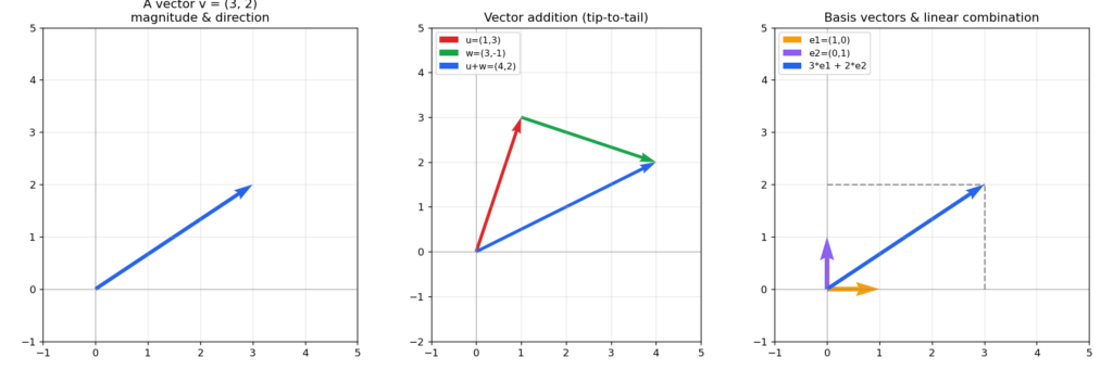
Left: a single vector as an arrow — magnitude and direction. Middle: tip-to-tail addition — $\mathbf{u}+\mathbf{w}$ is the arrow you get by walking $\mathbf{u}$, then $\mathbf{w}$, from the origin. Right: any vector as a weighted combination of the standard basis vectors $\mathbf{e}_1, \mathbf{e}_2$e1​,e2​ — the dashed lines show exactly how $3\mathbf{e}_1 + 2\mathbf{e}_2$3e1​+2e2​ reconstructs $(3,2)$(3,2), the same linear-combination idea from §1.4, made visible.

5. Where this leaves us

Every operation used informally across Modules 00 and 01 — cosine similarity, embedding averages, the attention weighting formula — is now standing on a precise, provable foundation rather than “code that happened to work.” That’s not a formality; it’s exactly the difference between recognizing an equation in a paper and having to guess at what it’s doing.

6. Before Episode 02.01

Every vector operation today involved exactly two vectors at a time — one dot product, one sum, one norm. But attention (Episode 01.02) computes a similarity score between one query and every key in a sentence simultaneously, all at once, not one pair at a time in a loop. What kind of mathematical object would let you express “many vectors, organized together, operated on all at once” as a single unit — and what operation would replace “a bunch of individual dot products” with one clean computation?

That question is the on-ramp into Episode 02.01 — matrices, and matrix multiplication as organized, simultaneous dot products.

Previous: Episode 01.02 — Toward Contextual Representations (Module 01 wrap) Next: Episode 02.01 — Matrices and the Geometry of Linear Transformations