The Vanishing Gradient Problem Explained: Why ReLU Replaced Sigmoid (Ep:03.02)

Views: 9

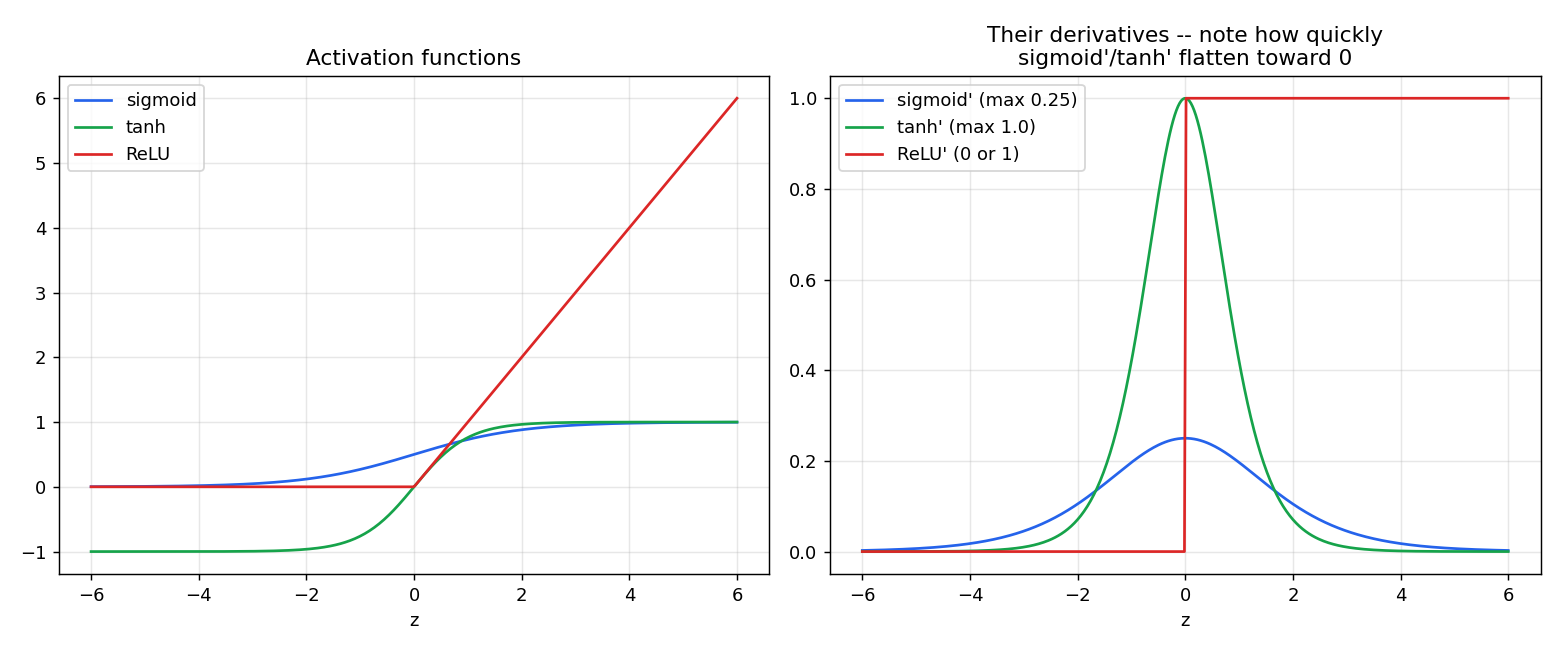
Sigmoid’s derivative maxes out at 0.25 and shrinks fast — multiply that through 15 layers and gradients vanish to nearly zero before reaching early layers. Module 3 of From Zero to Agents proves it, measures it in a real PyTorch network, and shows why ReLU fixed it.

Episode 03.01 ended by asking what sigmoid’s slope does far from zero, and what that might mean for gradients flowing through many stacked layers. The short answer: sigmoid’s slope collapses toward zero rapidly away from the origin, and when the chain rule (Episode 02.02 §1.5) multiplies many such near-zero slopes together across a deep network, the product can shrink to something computationally indistinguishable from zero — long before it reaches the earliest layers. This episode proves that precisely, measures it directly in a real trained network, and shows why a much simpler function eventually replaced sigmoid almost everywhere.

1. Theory: three activation functions, and the property that actually matters

1.1 Sigmoid. $\sigma(z) = \frac{1}{1+e^{-z}}$​, squashing any real number into $(0,1)$ — the same function used for turning attention/word2vec scores into probabilities back in Episode 00.03 and Episode 02.04. As an activation function inside a network (not just at the final output), it has a specific structural weakness worth naming directly: for $|z|$ large in either direction, the curve flattens almost completely — the function is said to saturate. A saturated neuron’s output barely changes no matter how its input changes, which — per §1.4 of this episode — is exactly the property that breaks deep training.

1.2 Tanh.$\tanh(z) = \frac{e^z – e^{-z}}{e^z+e^{-z}}$, squashing into $(-1,1)$ instead of $(0,1)$ — zero-centered, which turns out to help optimization somewhat (a detail Module 03 won’t dwell on, but real papers frequently mention it), and its derivative reaches a higher maximum than sigmoid’s. It still saturates at both extremes, though, inheriting the same core problem in a milder form.

1.3 ReLU — deliberately almost embarrassingly simple.$\text{ReLU}(z) = \max(0, z)$ (Nair & Hinton, 2010, though the underlying idea is older). For any positive input, it’s just the identity function — no squashing, no saturation, output keeps growing exactly as fast as input does. For any negative input, it’s flatly zero. This asymmetry is the entire point, made precise in §2.

1.4 The vanishing gradient problem, in plain language before the math. Backpropagation, per Episode 02.02 §1.5/§3, computes a weight’s effect on the final loss by multiplying together a chain of local derivatives, one per layer, from the output back to that weight. If every one of those local derivatives is comfortably less than 1 (as sigmoid’s always is — see §2.1), multiplying many of them together shrinks the product geometrically with depth — exactly the same mathematical shape as Episode 02.03‘s convergence analysis, just working against you this time instead of for you. By the time that chain reaches an early layer in a genuinely deep network, the gradient signal can become so small it’s effectively zero — the early layers stop receiving any meaningful information about how to improve, and training stalls, even though later layers might still be learning fine.

2. Math: deriving the derivatives, and quantifying the shrinkage exactly

2.1 Sigmoid’s derivative, and its hard ceiling. A clean derivation (via the quotient rule, which we won’t belabor) gives:

$$\sigma'(z) = \sigma(z)\big(1-\sigma(z)\big)$$

This has a maximum you can find directly: $\sigma(z)(1-\sigma(z))$ is a product of two numbers that always sum to 1 (since $\sigma(z) \in (0,1)$), and a product of two positive numbers with a fixed sum is maximized when they’re equal — at $\sigma(z)=0.5$, exactly $z=0$. Plugging in: $0.5 \times 0.5 = 0.25$. Sigmoid’s derivative can never exceed 0.25 0.25, anywhere, for any input — and it decays toward zero rapidly as $|z|$ grows past a few units.

2.2 Quantifying the chain-rule shrinkage exactly. Suppose, optimistically, every layer in a deep sigmoid network happens to sit right at sigmoid’s best possible derivative, $0.25$ (in practice it’s usually worse than this). For a network $L$ layers deep, the chain rule multiplies roughly $L$ such terms together:$$\prod_{l=1}^{L} \sigma'(z^{(l)}) \leq (0.25)^L$$

For $L=10$: $(0.25)^{10} \approx 9.5 \times 10^{-7}$ — under one part in a million, in the best case. For $L=15$, deeper still: $(0.25)^{15} \approx 9 \times 10^{-10}$. This is not a pathological edge case — it’s the optimistic bound, assuming every single neuron sits exactly at its point of maximum sensitivity, which real, randomly-initialized networks essentially never do in practice. Section 4 measures the real number in an actual network, not just this idealized bound.

2.3 Why ReLU avoids this — and its own, different problem. ReLU’s derivative is exactly $1$ for any positive input, and exactly $0$ for any negative input (technically undefined at exactly $z=0$; frameworks conventionally treat it as $0$ or $1$ there). For the chain of active (positive-input) neurons, the chain-rule product in §2.2 becomes a product of $1$s — no shrinkage at all, regardless of depth. This is the direct fix for vanishing gradients through active paths. The trade-off, sometimes called the “dying ReLU” problem: a neuron whose input is always negative for every training example has a permanently zero gradient and can stop learning entirely, forever — a different failure mode, milder in practice, and the reason variants like Leaky ReLU (allowing a small non-zero slope for negative inputs, e.g. $0.01z$ instead of flat $0$) exist.

3. Decoding real notation — how papers describe this

Papers discussing this issue (notably Glorot & Bengio’s 2010 analysis of why deep networks were historically hard to train, and Nair & Hinton’s 2010 ReLU paper) typically write the backpropagated gradient through a chain of layers as a product of Jacobians or, in the simplified scalar case we’ve been using, a product like $\prod_{l} \sigma'(z^{(l)})$ — exactly the expression in §2.2. Recognizing this product-of-derivatives structure on sight is the whole skill: whenever a paper’s argument hinges on “the gradient vanishes/explodes with depth,” it is, structurally, always this same multiplication — many numbers, each less than (or greater than) 1, multiplied together enough times to shrink toward zero (vanishing) or blow up toward infinity (exploding) — the same geometric-sequence mathematics from Episode 02.03, now applied across layers instead of across training steps.

4. Code: the derivatives, verified, and the vanishing gradient measured directly

4.1 From scratch — all three activations and their derivatives, verified against autograd

import numpy as np

def sigmoid(z): return 1 / (1 + np.exp(-z))
def sigmoid_deriv(z):
    s = sigmoid(z)
    return s * (1 - s)

zs = np.array([-5, -2, -0.5, 0, 0.5, 2, 5], dtype=float)
print("sigmoid'(z):", np.round(sigmoid_deriv(zs), 4))
print("max possible sigmoid':", sigmoid_deriv(np.array([0.0]))[0])

sigmoid'(z): [0.0066 0.105  0.235  0.25   0.235  0.105  0.0066]
max possible sigmoid': 0.25

Exactly matching §2.1’s derived ceiling of $0.25$ at $z=0$, and already visibly small ($0.0066$) by $z=\pm5$ — a moderately large input is enough to nearly kill the gradient passing through that single neuron.

import torch
zt = torch.tensor(zs, requires_grad=True)
torch.sigmoid(zt).sum().backward()
print("torch gradient:", np.round(zt.grad.numpy(), 4))
print("matches manual derivative?", np.allclose(zt.grad.numpy(), sigmoid_deriv(zs), atol=1e-4))

torch gradient: [0.0066 0.105  0.235  0.25   0.235  0.105  0.0066]
matches manual derivative? True

4.2 Measuring vanishing gradients directly, in a real 15-layer network

import torch.nn as nn

def build_deep_net(activation_cls, n_layers=15, width=20):
    layers = []
    for _ in range(n_layers):
        layers += [nn.Linear(width, width), activation_cls()]
    layers.append(nn.Linear(width, 1))
    return nn.Sequential(*layers)

def report(name, activation_cls):
    torch.manual_seed(0)
    net = build_deep_net(activation_cls)
    x = torch.randn(1, 20)
    loss = (net(x) - torch.tensor([[1.0]]))**2
    loss.backward()
    grad_norms = [m.weight.grad.norm().item() for m in net if isinstance(m, nn.Linear)]
    print(f"{name}: layer 0 (near input) grad = {grad_norms[0]:.2e}   layer 15 (near output) grad = {grad_norms[-1]:.2e}")
    print(f"  ratio (input-layer / output-layer): {grad_norms[0]/grad_norms[-1]:.2e}")

report("Sigmoid, 15 layers", nn.Sigmoid)
report("ReLU, 15 layers", nn.ReLU)

Sigmoid, 15 layers: layer 0 (near input) grad = 0.00e+00   layer 15 (near output) grad = 5.39e+00
  ratio (input-layer / output-layer): 5.47e-14

ReLU, 15 layers: layer 0 (near input) grad = 2.29e-05   layer 15 (near output) grad = 1.16e+00
  ratio (input-layer / output-layer): 1.97e-05

This is the vanishing gradient problem, measured directly in a real (if untrained-so-far) network, not simulated: in the 15-layer sigmoid network, the gradient reaching the layer nearest the input is about 5×10−14 times smaller than the gradient at the output layer — for practical purposes, zero; that layer would receive essentially no training signal at all. The identically-structured ReLU network’s input-layer gradient is roughly $10^{-5}$ times its output layer’s — still shrinking with depth (a real, separate phenomenon worth its own future episode), but nine orders of magnitude better preserved than sigmoid’s, purely from swapping the activation function and changing nothing else about the architecture.

5. Where this leaves us

We now have the actual, quantified reason ReLU (and its variants) displaced sigmoid as the default choice for hidden layers in deep networks — not a stylistic preference, a direct, measurable consequence of §2.1’s $0.25$ ceiling compounding across depth via the exact chain-rule mechanism Module 02 built. Sigmoid and tanh remain useful — at output layers specifically, where their bounded range is exactly what’s needed (a probability between 0 and 1, for instance) — but as the repeated activation inside a deep stack of hidden layers, the vanishing-gradient math makes the case for ReLU-family functions directly, without appeal to intuition.

6. Before Episode 03.03

Every network built so far in this module — the hand-constructed XOR solver, the trained 2-layer network, today’s 15-layer gradient experiment — used weights either hand-set or drawn from PyTorch’s default random initialization, without asking whether that starting point matters. Given what §4.2 just showed about gradients shrinking or growing across layers depending on the activation function used, what do you think happens if a deep network’s initial weights are drawn from a poorly-chosen distribution — too large, or too small — before training even begins?

That’s the on-ramp into Episode 03.03 — weight initialization, and why it turns out to matter just as much as the activation function itself.

Previous: Episode 03.01 — Multi-Layer Perceptrons and Solving XOR Next: Episode 03.03 — Weight Initialization and Why It Matters