The Perceptron and the XOR Problem: Why Single Neurons Aren’t Enough (Ep:03.00)

Views: 11

In 1969, Minsky and Papert proved a single perceptron can never learn XOR. Module 3 of From Zero to Agents derives that proof from scratch, trains a real perceptron in Python, and shows exactly why it fails — and why that failure demands multi-layer networks.

Module 02 built every mathematical tool a neural network needs: vectors, matrices, gradients, convergence, probability. Module 03 assembles them into the actual thing — starting with the smallest possible unit, and, deliberately, starting with a real historical failure. Frank Rosenblatt introduced the perceptron in 1958 as a simple model of a biological neuron, and it genuinely worked for a range of problems. Then, in 1969, Marvin Minsky and Seymour Papert proved — rigorously, not empirically — that it fundamentally couldn’t solve a specific, embarrassingly simple problem. That proof (which we’ll redo ourselves in §2) is widely credited with contributing to the first “AI winter,” a period of collapsed funding and interest in neural networks that lasted over a decade. Understanding exactly what broke, and why, is the fastest route to understanding why every network built from here forward looks the way it does.

1. Theory: the simplest possible artificial neuron

1.1 What a perceptron computes. A perceptron takes a vector of inputs $\mathbf{x}$, computes a weighted sum plus a bias term (this is exactly the matrix-vector operation from Episode 02.01, with a single output row), and passes the result through a step function: output $1$ if the sum is at or above zero, output $0$ otherwise. Geometrically, $\mathbf{w}\cdot\mathbf{x}+b = 0$ defines a straight line (in 2D) or a flat plane (in higher dimensions) — everything on one side of that line gets classified as $1$, everything on the other side as $0$. This kind of decision boundary is called linear, and a perceptron can learn any problem where a single straight line correctly separates the two classes — no more, no less.

1.2 Two examples that work. The logical AND function: output $1$ only if both inputs are $1$. Plot the four input pairs $(0,0), (0,1), (1,0), (1,1)$ with their correct outputs, and a single straight line genuinely does separate the single positive case $(1,1)$ from the other three. The logical OR function behaves the same way — one straight line separates the single negative case $(0,0)$ from the rest. Both are called linearly separable for exactly this reason.

1.3 The example that doesn’t work — XOR. The logical XOR (“exclusive or”): output $1$ if the inputs differ, $0$ if they’re the same. Plot it: $(0,0)\to 0$, $(0,1)\to 1$, $(1,0)\to 1$, $(1,1)\to 0$. Try to draw a single straight line separating the two 1-outputs from the two 0-outputs — it can’t be done; the positive cases sit on opposite corners of the square, with a negative case wedged directly between them on both diagonals. No single perceptron, trained however long, however cleverly, can ever solve this. Section 2 proves this isn’t a training difficulty — it’s a mathematical impossibility.

1.4 Why this matters more than a curiosity. XOR isn’t an obscure edge case invented to break the model — it’s representative of an enormous class of real problems where the correct decision genuinely depends on a combination of factors, not a simple weighted threshold. The Minsky-Papert result forced the field to confront that a single neuron’s expressive power is fundamentally limited — and pointed directly at the fix, which is where this episode ends and Episode 03.01 begins.

2. Math: proving AND works and XOR doesn’t

2.1 The perceptron function, precisely.

$$\hat{y} = \text{step}(\mathbf{w}\cdot\mathbf{x} + b), \qquad \text{step}(z) = \begin{cases} 1 & z \geq 0 \\ 0 & z < 0 \end{cases}$$

2.2 Proving AND is solvable — by exhibiting a working solution.

Claim: $w_1=1, w_2=1, b=-1.5$ solves AND. Check all four cases directly:

• $(0,0)$: $1(0)+1(0)-1.5 = -1.5 < 0 \to 0$ ✓.
• $(0,1)$: $1(0)+1(1)-1.5 = -0.5 < 0 \to 0$ ✓.
• $(1,0)$: same as above by symmetry, $\to 0$→0 ✓.
• $(1,1)$: $1(1)+1(1)-1.5 = 0.5 \geq 0 \to 1$ ✓.

All four match the truth table. A working solution exists — AND is provably linearly separable, by construction.

2.3 Proving XOR is unsolvable — by contradiction.

Suppose, for contradiction, that some $w_1, w_2, b$ correctly solves XOR. The four required conditions, directly from the step function’s definition (using $\geq 0 \Rightarrow$ output 1, and $<0 \Rightarrow$ output 0):$$b < 0 \quad \text{(from } (0,0)\to 0\text{)}$$$$w_2 + b \geq 0 \quad \text{(from } (0,1) \to 1\text{)}$$$$w_1 + b \geq 0 \quad \text{(from } (1,0) \to 1\text{)}$$$$w_1 + w_2 + b < 0 \quad \text{(from } (1,1) \to 0\text{)}$$

Add the second and third inequalities together: $w_1 + w_2 + 2b \geq 0$. Now compare this to the fourth inequality, $w_1+w_2+b<0$. Subtract the fourth from the combined result: $(w_1+w_2+2b) – (w_1+w_2+b) \geq 0 – (\text{something} < 0)$, which simplifies to $b > -b$, i.e. $2b > 0$, i.e. $b > 0$. But the first condition required $b < 0$. $b$ cannot be simultaneously greater than zero and less than zero — a direct contradiction. No values of $w_1, w_2, b$ exist that satisfy all four conditions at once. XOR is not linearly separable, full stop, proven algebraically rather than by exhausting every possible weight (which wouldn’t even be possible, since weights are continuous).

2.4 A problem inherited from Module 02 — the step function’s derivative. There’s a second, independent problem with the perceptron worth flagging now, because it’s exactly the machinery Module 02 spent five episodes building: the step function’s derivative is zero everywhere except at the single point $z=0$, where it’s undefined entirely (an instantaneous jump has no meaningful slope). Recall Episode 02.02 — gradient descent needs a derivative that actually carries information about which direction to adjust weights. A derivative that’s zero almost everywhere gives gradient descent nothing to work with. This is precisely why Rosenblatt’s original training rule (§3) wasn’t gradient descent at all — it predates that formalization for neural networks — and it’s precisely why every practical activation function used from here forward (sigmoid, ReLU, and others, arriving in Episode 03.01) is chosen specifically to have a well-behaved, non-zero derivative almost everywhere.

3. A real historical equation — the original perceptron learning rule

Rosenblatt’s 1958 update rule, in something close to its original notation:

$$\mathbf{w} \leftarrow \mathbf{w} + \eta\,(y – \hat{y})\,\mathbf{x}, \qquad b \leftarrow b + \eta\,(y-\hat{y})$$

Decoded: $y$ is the true label, $\hat{y}$​ the current prediction, $\eta$ a learning rate. If the prediction is already correct, $y-\hat{y}=0$ and nothing changes. If the model predicted $0$ but the truth was $1$ (undershooting), $y-\hat{y}=1$, and the weights get nudged in the direction of $\mathbf{x}$ — making that same input more likely to cross the threshold next time. If it overshot, weights get nudged the opposite way. This isn’t gradient descent on a smooth loss (the step function has no usable gradient, per §2.4) — it’s a direct, hand-designed correction rule that happens to behave similarly to gradient descent’s “predicted minus true” pattern from Episode 02.04‘s cross-entropy result, arrived at independently, three decades earlier, by different reasoning entirely. Worth recognizing on sight: this exact $(y-\hat{y})$ structure recurs throughout the history of learning rules, under different names, because it’s the simplest possible encoding of “correct the error in the direction that would have fixed it.”

4. Code: building a perceptron, watching it succeed and fail exactly as proven

4.1 From scratch

import numpy as np

def step(z):
    return 1 if z >= 0 else 0

class Perceptron:
    def __init__(self, n_inputs, lr=0.1):
        self.w = np.zeros(n_inputs)
        self.b = 0.0
        self.lr = lr

    def predict(self, x):
        return step(np.dot(self.w, x) + self.b)

    def train(self, X, y, epochs=20):
        history = []
        for _ in range(epochs):
            errors = 0
            for xi, yi in zip(X, y):
                update = self.lr * (yi - self.predict(xi))   # exactly Rosenblatt's rule, §3
                self.w += update * xi
                self.b += update
                errors += int(update != 0.0)
            history.append(errors)
            if errors == 0:
                break
        return history

X = np.array([[0,0],[0,1],[1,0],[1,1]])

p_and = Perceptron(2)
print("AND errors per epoch:", p_and.train(X, np.array([0,0,0,1]), epochs=20))
print("AND learned weights:", p_and.w, "bias:", p_and.b)

p_xor = Perceptron(2)
print("\nXOR errors per epoch:", p_xor.train(X, np.array([0,1,1,0]), epochs=50))

AND errors per epoch: [2, 3, 3, 0]
AND learned weights: [0.2 0.1] bias: -0.2

XOR errors per epoch: [3, 3, 4, 4, 4, 4, 4, 4, 4, 4, 4, 4, 4, 4, 4, 4, 4, 4, 4, 4, 4, 4, 4, 4, 4, 4, 4, 4, 4, 4, 4, 4, 4, 4, 4, 4, 4, 4, 4, 4, 4, 4, 4, 4, 4, 4, 4, 4, 4, 4]

AND converges to zero errors in four epochs, matching §2.2’s proof — a solution genuinely exists, and Rosenblatt’s rule finds one. XOR runs for the full 50 epochs and never drops below 4 misclassified errors per epoch — not because the training ran too briefly or the learning rate was wrong, but because §2.3 proved no solution exists for it to converge to, no matter how long it runs.

4.2 Using a library — sklearn, confirming the identical result

from sklearn.linear_model import Perceptron

clf_and = Perceptron(max_iter=1000).fit(X, [0,0,0,1])
print("AND accuracy:", clf_and.score(X, [0,0,0,1]))   # 1.0

clf_xor = Perceptron(max_iter=1000).fit(X, [0,1,1,0])
print("XOR accuracy:", clf_xor.score(X, [0,1,1,0]))   # 0.5 -- chance level

AND accuracy: 1.0
XOR accuracy: 0.5

A production-grade, heavily-optimized implementation, given a thousand training iterations to work with, still only reaches 50% accuracy on XOR — exactly chance level for a binary problem. This isn’t an implementation limitation of sklearn. It’s the same mathematical impossibility from §2.3, confirmed by a completely independent codebase.

4.3 Seeing why, geometrically

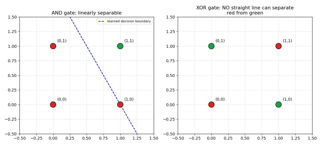
Left: AND’s four points, with the actual line the perceptron learned (from §4.1’s weights) cleanly separating the single green point from the three red ones. Right: XOR’s four points — no straight line, drawn any direction, at any angle, can put both green points on one side and both red points on the other. The green points sit on one diagonal, the red points on the other; separating them requires a bend, not a line.

5. Where this leaves us

A single perceptron is provably limited to problems a straight line (or flat plane, in higher dimensions) can solve. That’s not a training failure to be fixed with more epochs, a better learning rate, or more data — it’s a structural ceiling on what one linear unit can ever represent, proven algebraically in §2.3 and confirmed by two independent implementations in §4.

6. Before Episode 03.01

XOR needs a bent decision boundary, not a straight one. A single perceptron draws exactly one straight line. What would it take to combine multiple perceptrons — each one still just drawing its own straight line — into a system capable of representing a bent, non-linear boundary overall? Think geometrically: if one perceptron can carve the input space into “left of this line” and “right of this line,” what happens if you feed the output of several perceptrons into another perceptron as its input?

That question is the entire idea behind the multi-layer perceptron — the actual first “deep” network — and it’s where Episode 03.01 picks up.

Previous: Module 02, Episode 02.04 — Probability, Softmax, and Cross-Entropy (Module 02 wrap) Next: Episode 03.01 — Multi-Layer Perceptrons and Solving XOR