Positional Encoding Explained: How Transformers Learn Word Order (Ep:04.04)

Views: 1

Attention is mathematically blind to sequence order — swap two tokens and every output is just the same values, permuted. Module 4 of From Zero to Agents derives sinusoidal positional encoding, proves its relative-position property with trigonometric identities, and demonstrates the permutation-blindness directly in code.

Episode 04.03 ended with a genuinely surprising fact: the transformer block built and verified across that entire episode cannot tell “the cat sat” from “sat the cat.” Attention computes pairwise relationships purely from content — swap two input tokens, and every $QK^T$ score, every attention weight, every output value stays exactly the same, just relabeled to the new positions. This episode proves that precisely, then fixes it — not by changing the architecture, but by changing what goes into it.

1. Theory: why attention is permutation-blind, and where the fix has to live

1.1 The precise reason, revisited. Recall Episode 02.01 §2.4: $QK^T$‘s entry $(i,j)$ is $\text{row}_i(Q)\cdot\text{row}_j(K)$ — a similarity score computed purely from the content of positions $i$ and $j$, with no reference anywhere to what $i$ and $j$ actually are as sequence positions. Permute the rows of the input, and you get exactly the same set of pairwise scores, just relabeled — the entire computation is, in the technical sense, permutation-equivariant: shuffle the input, get an identically-shuffled output, with no new information distinguishing the orderings. Section 4 demonstrates this is not a theoretical nitpick — it’s measurable, exactly, in real code.

1.2 Why the fix can’t live in the attention mechanism itself. This permutation-equivariance isn’t a bug to patch inside attention — it’s a direct, unavoidable consequence of what a dot product is (Episode 02.00 §2.2): a similarity measure between two vectors’ content, with no built-in notion of “where” either vector came from. The fix has to happen before attention ever runs: inject position information directly into each token’s own vector, so that “content” and “position” become inseparably part of the same input, and the dot-product similarity attention computes automatically reflects both.

1.3 The chosen solution — sinusoidal positional encoding. Vaswani et al. (2017) chose a specific, fixed (not learned) scheme: generate a unique vector for every position using sine and cosine waves of different frequencies, and simply add this vector to each token’s embedding before it ever reaches an attention layer. The intuition worth building before the formula: think of how binary numbers represent position — the lowest bit flips every step, the next bit every two steps, the next every four, and so on, with each bit oscillating at half the frequency of the one before it. Sinusoidal encoding is a smooth, continuous cousin of exactly this idea: each pair of embedding dimensions oscillates at its own fixed frequency, low dimensions cycling quickly, high dimensions cycling slowly, together giving every position a unique, learnable “fingerprint” across the full embedding width.

2. Math: the formula, and the property that makes it genuinely clever

2.1 The sinusoidal formula, precisely. For position $\text{pos}$pos and dimension index $2i$ or $2i+1$ (dimensions are handled in sine/cosine pairs):

$$PE_{(\text{pos}, 2i)} = \sin\left(\frac{\text{pos}}{10000^{2i/d_{\text{model}}}}\right), \qquad PE_{(\text{pos}, 2i+1)} = \cos\left(\frac{\text{pos}}{10000^{2i/d_{\text{model}}}}\right)$$

Read the structure: each dimension pair $(2i, 2i+1)$ shares a frequency, $1/10000^{2i/d_{\text{model}}}, that shrinks as $i grows — dimension pair 0 oscillates fastest (period near $2\pi), the last dimension pair oscillates slowest (period near $10000 \times 2\pi ). Every position gets a $d_{\text{model}}$dmodel​-dimensional vector, and because different dimension pairs cycle at wildly different rates, the combination of all of them together uniquely identifies each position, exactly like the binary-counting analogy in §1.3.

2.2 The property that makes this specific choice more than an arbitrary fingerprint.Here’s the genuinely clever part, provable directly from basic trigonometric identities. Using the angle-addition formulas $\sin(a+b) = \sin a\cos b + \cos a \sin b$ and $\cos(a+b) = \cos a \cos b – \sin a \sin b$, for any fixed offset $k$k, the encoding at position $\text{pos}+k$ can be written as a linear function of the encoding at position $\text{pos}$ — specifically, a rotation:

$$\begin{pmatrix}PE_{(\text{pos}+k, 2i)} \\ PE_{(\text{pos}+k, 2i+1)}\end{pmatrix} = \begin{pmatrix}\cos(k\omega_i) & \sin(k\omega_i) \\ -\sin(k\omega_i) & \cos(k\omega_i)\end{pmatrix}\begin{pmatrix}PE_{(\text{pos}, 2i)} \\ PE_{(\text{pos}, 2i+1)}\end{pmatrix}$$

where $\omega_i$ is that dimension pair’s frequency from §2.1. Crucially, this rotation matrix depends only on the offset $k$, not on the absolute position $\text{pos}$pos itself. This means, in principle, a network’s learned weights (specifically, inside $W_Q$​ or $W_K$​, Episode 04.02 §1.2) could implement “attend to the token 3 positions back” as a fixed linear operation applicable everywhere in the sequence, rather than needing to separately learn “3 positions back” for every possible absolute starting position. This is a genuine mathematical convenience of the sinusoidal scheme specifically — not a property every possible positional encoding scheme would automatically have.

2.3 Combining position with content — addition, not concatenation. The actual input to the first transformer block is simply $\mathbf{x}_{\text{pos}} = \text{TokenEmbedding}(\text{token}) + PE_{\text{pos}}$ — the positional vector is added directly on top of the token’s embedding, not appended alongside it as extra dimensions. This is a real, slightly counterintuitive design choice worth naming: nothing forces “what token” and “where” to be added together cleanly, but in practice, sufficiently high-dimensional spaces have enough room for the network’s learned projections to separate the two signals back out where needed, and the sum keeps the embedding dimensionality unchanged rather than growing it — a genuine engineering trade-off, not a mathematical necessity.

3. Decoding real notation — and the alternative you’ll also see constantly

The formula in §2.1 is stated close to verbatim in Vaswani et al.’s original paper, §3.5. The other extremely common choice, used in GPT and BERT-family models, is simpler to state and easy to recognize: a learned positional embedding — literally another embedding table (Episode 02.01 §2.2’s exact mechanism), indexed by position instead of by token identity, with the position vectors learned via ordinary backpropagation rather than fixed by a formula. The trade-off worth knowing: sinusoidal encoding, being a formula rather than a lookup table, can in principle be evaluated at any position, including ones longer than anything seen in training — genuine length generalization. A learned positional embedding table has a fixed maximum size and, without special handling, simply has nothing to output for a position beyond what it was trained on. Seeing either approach named in a paper’s architecture section — “sinusoidal” versus “learned absolute positional embeddings” — is describing exactly this trade-off, not two unrelated ideas.

4. Code: the permutation-blindness proven, the fix verified, the rotation property confirmed

4.1 Proving the permutation-blindness directly

import torch
from previous_episode import MultiHeadAttention   # Episode 04.03's implementation, unchanged

mha = MultiHeadAttention(d_model=8, num_heads=2)
torch.manual_seed(1)
A, B, C = torch.randn(1,8), torch.randn(1,8), torch.randn(1,8)

seq_ABC = torch.stack([A,B,C], dim=1)
seq_CBA = torch.stack([C,B,A], dim=1)   # same tokens, fully reversed order

with torch.no_grad():
    out_ABC = mha(seq_ABC)
    out_CBA = mha(seq_CBA)

print("Is reversed-input output just the original output, reversed?",
      torch.allclose(out_CBA[0], out_ABC[0].flip(0), atol=1e-5))

Is reversed-input output just the original output, reversed? True

Exactly as §1.1 predicted: feeding the tokens in reverse order produces exactly the same three output vectors, just in reversed order — the network computed nothing genuinely different; it just relabeled which output belongs to which position.

4.2 Generating sinusoidal encoding, and confirming it breaks the symmetry

def sinusoidal_pe(seq_len, d_model):
    pe = torch.zeros(seq_len, d_model)
    position = torch.arange(seq_len).unsqueeze(1).float()
    div_term = 10000 ** (torch.arange(0, d_model, 2).float() / d_model)
    pe[:, 0::2] = torch.sin(position / div_term)
    pe[:, 1::2] = torch.cos(position / div_term)
    return pe

pe = sinusoidal_pe(3, 8).unsqueeze(0)
with torch.no_grad():
    out_ABC_pe = mha(seq_ABC + pe)
    out_CBA_pe = mha(seq_CBA + pe)

print("With positional encoding, is it still just a reversal?",
      torch.allclose(out_CBA_pe[0], out_ABC_pe[0].flip(0), atol=1e-5))

With positional encoding, is it still just a reversal? False

The moment position information is added to the input, the symmetry genuinely breaks — the network’s output for “A, B, C” and “C, B, A” are no longer simple reversals of each other, because the network now has a real signal distinguishing “first position” from “last position,” independent of which token happens to sit there.

4.3 Confirming the relative-position rotation property from §2.2

import numpy as np

d_model, i, k = 8, 1, 3   # test dimension pair i=1, offset k=3
freq = 1 / (10000 ** (2*i/d_model))

def rotation_matrix(k, freq):
    theta = k * freq
    return np.array([[np.cos(theta), np.sin(theta)], [-np.sin(theta), np.cos(theta)]])

R = rotation_matrix(k, freq)
for pos in [0, 2, 5, 7]:
    pe_pos = np.array([np.sin(pos*freq), np.cos(pos*freq)])
    pe_pos_plus_k = np.array([np.sin((pos+k)*freq), np.cos((pos+k)*freq)])
    predicted = R @ pe_pos
    print(f"pos={pos}: actual={np.round(pe_pos_plus_k,4)}  R@PE(pos)={np.round(predicted,4)}  match={np.allclose(pe_pos_plus_k, predicted)}")

pos=0: actual=[0.2955 0.9553]  R@PE(pos)=[0.2955 0.9553]  match=True
pos=2: actual=[0.4794 0.8776]  R@PE(pos)=[0.4794 0.8776]  match=True
pos=5: actual=[0.7174 0.6967]  R@PE(pos)=[0.7174 0.6967]  match=True
pos=7: actual=[0.8415 0.5403]  R@PE(pos)=[0.8415 0.5403]  match=True

The same rotation matrix $R$R — built once, from only the offset $k=3$k=3 and the frequency, with no dependence on pos — correctly transforms PE(pos) into PE(pos+3) for every tested starting position. This confirms §2.2’s claim exactly, not just algebraically: relative position really is a fixed linear transformation under this specific encoding scheme.

4.4 Seeing the encoding directly

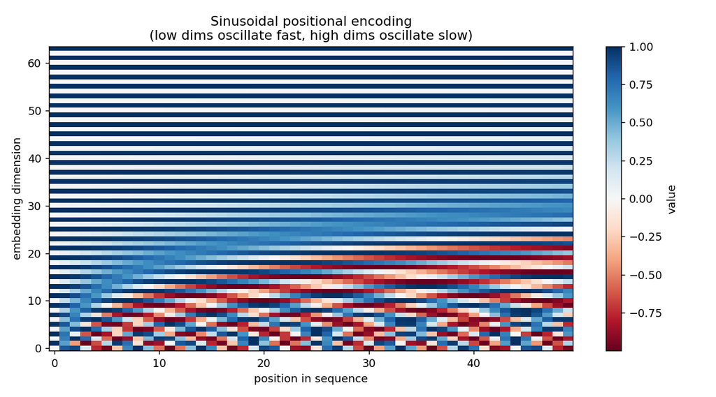
Each row is one sequence position; each column is one embedding dimension. Low-index dimensions (left) oscillate rapidly across positions; high-index dimensions (right) barely change over the visible range — precisely the “fast bit, slow bit” structure from §1.3’s binary-counting analogy, made visible.

5. Where this leaves us

A shape-preserving, provably permutation-blind mechanism has been given a real, mathematically well-behaved sense of order — not by touching the attention computation at all, but by making sure position is already baked into what attention receives as input. With this piece in place, every component needed for a complete, working transformer encoder has now been built, derived, and verified from first principles: tokenization and embeddings (Module 01), the full neural network toolkit (Module 03), and now sequence-processing with genuine, trainable relevance and genuine order-awareness (Module 04).

6. Before Episode 04.05

Everything built this module processes a sequence and produces a same-length sequence of contextualized vectors — useful for understanding a sequence, but not yet for generating one token at a time, the way a language model actually produces text. If a model is predicting the next token, what would go wrong if a position were allowed to attend to tokens that come after it in the sequence — tokens it wouldn’t actually have access to yet at generation time? What change to the attention computation itself would prevent that?

That’s the on-ramp into Episode 04.05 — causal masking, and finally assembling a complete, generative, GPT-style architecture end to end.

Previous: Episode 04.03 — Multi-Head Attention and the Transformer Block Next: Episode 04.05 — Causal Masking and a Complete GPT-Style Model